Exercise 1: Ultrasound image display

Monday, September 11, 14.30-17.00 in the E-databar, build 341, ground floor, room 015.

Purpose:

The purpose of this exercise is to demonstrate the signal processing involved in ultrasound image display. This includes finding the enveloped through a Hilbert transform, compressing the data, and making the image interpolation. It also show how serveral frames can be combined into one movie.

Preparation:

Read Chapter 2 in the book: Jørgen Arendt Jensen: Estimation of Blood Velocities Using Ultrasound, A Signal Processing Approach, Cambridge University Press, 1996.

Go through the different exercise points and write down suggestions for your Matlab code.

Hints using Matlab:

Write all Matlab instructions in a file (f. ex. ex1.m) and run the file in the Matlab window by typing ex1 at the Matlab prompt. With this approach you will be able to receive help from the instructor about problems with your code.

The data files can also been found on DTU Inside under exercise1. This can be used, if you have problems downloading the files from this page.

Exercise:

1. Log in to one of the PCs. Make a directory course_31545, where all the course files can be stored.

2. Start a web browser and go to the course home page at:

   https://courses.healthtech.dtu.dk/22485
   

   Go to exercise1 (this page at: https://courses.healthtech.dtu.dk/22485/?exercises/exercise1/exercise1.html) and download the image data by right-clicking here. Place the datafile with the name rf_data_phantom.mat in your directory for the course.

   Load the data into Matlab and look at the variables by writing whos. The following variables are found in the file:

   Variable name	Content	Unit
   RFdata	The measured RF data from the transducer after TGC amplification. The matrix contains one column for each of the lines in the image. The data is 16 bits, two-complements integers, where a full range value of 32768 corresponds to 2 volts.	v
   fs	Sampling frequency	Hz
   start_of_data	Starting depth for data	m
   start_angle	Starting angle for data	rad
   angle	Angle between the different RF lines	rad
   c_sound	Speed of sound	m/s
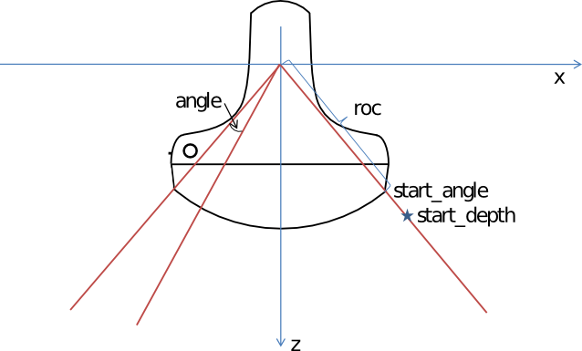
   roc	Radius of curvature. Distance from (0,0) to the patient side of the transducer.	m

   
   

   The variables are defined in the figure below:
   
   

   
   
   

   Plot the values for the center RF line in the image with the correct depth scaling on the x-axis.  Use the sampling frequency, start depth and speed of sound for generating the correct depth values.  Note that the rf_data is int16 and should be converted to double before they can be used.

3. Find the envelope of the data by making a Hilbert transform on each of the RF signals (see help hilbert). Check the envelope by plotting both a single RF signal and the envelope on top of each other.

4. Compress the envelope data to have a dynamic range of 60 dB and scale it to lie from 0 to 127 for a colormap with 128 gray level values.

5. Download the display programs (fast_int_uint32.mexa64 for Linux, fast_int_uint32.mexmaci64 in for_mac_matlab_2017 for Mac, or fast_int_unit32.mexw64 for windows, and make_interpolation.m, make_tables.m) from the zip filke: https://courses.healthtech.dtu.dk/22485/exercises/exercise1/programs/interpolation_programs.zip and put them in the short course directory. Use the routines make_tables and make_interpolation  to perform the polar to rectangular interpolation of the data. Write help make_tables and help make_interpolation to find out how the routines are used.

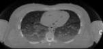
6. Make the interpolation for all image files 8820e_B_mode_invivo_frame_no_<XX> where <XX> is from 1 to 66. Each files houses an image like the one described above. All files are found in the zip-archive: in_vivo_data.zip. The images can be combined into a movie by the Matlab commands avifile and addframe (see the Matlab help for more information). The movie can be played by the command movie. The frame rate i 22 fr/s.