Exercise 4: Acquisition of spectral data and implementation of spectral estimation
Monday, October 2, 14.30-17.00 in the
E-databar, build 341, ground floor.
The purpose of this exercise is to demonstrate the signal processing involved
in a pulse wave velocity system. The processing is tried on both simulated
and in-vivo data.
Preparation:
Read Chapter 5 and 6 in the book: Jørgen Arendt Jensen: Estimation
of Blood Velocities Using Ultrasound, A Signal Processing Approach, Cambridge
University Press, 1996.
Go through the different exercise points and write down suggestions for
your Matlab code.
Exercise:
-
Make a Matlab procedure for calculating and displaying the spectrogram
of the demodulated ultrasound signal. The procedure should take the complex
signal data and divide it into overlapping segments using a Hanning window
and then perform a Fourier transform for finding the power spectrum.
The size of the segments should be selectable as well as the percentage
of overlap. The results should be displayed as a gray level spectrogram as
shown below:
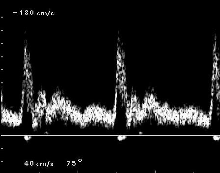
Figure 1: Spectrogram for carotid artery.
Use the Matlab command image and colomap(gray(128)) to make the display
with a dynamic range of 30 dB. Ensure that you have the proper units on
the axis: time on the x-axis and velocity on the
y-axis. Remember that complex data can have a power density spectrum,
where there is no symmetry around f=0 .
-
Download the data from the flow phantom from the web. The data is
described on the page: pht_audio.html
and the data file can be found at: data/pht_center1.mat
(You can also access these links through the web-page for this exercise
at:
https://courses.healthtech.dtu.dk/22485/?exercises/exercise4/exercise4.html)
The variable complex_data contains the complex data, forward
is the forward flow signal, and reverse is the reverse flow signal.
Use your program to find the spectrogram of the complex data with 128 sample
segments and calculation of a new spectrum every 5 ms. Which flow type is
this? Make a plot of the spectrogram for your report. Can this flow type
be found in the body?
-
Download data from the carotid artery. The data is described on the
page: ult_au_car.html
and the data file can be found at:
exercises/exercise4/data/pm_car1.mat
The variable complex_data contains the complex data, forward
is the forward flow signal, and reverse is the reverse flow signal.
Use your program to find the spectrogram of the complex data with 128 sample
segments and 5 ms between the segments. Make a plot of the spectrogram for
the report. Compare with Fig. 1 above. Do you get roughly
the same appearance?
-
Try with other data sets from the web. You can use data from the
aorta
or the portal vein.
You can find a description of the data at the page for the measured ultrasound
audio data:
https://courses.healthtech.dtu.dk/22485/?ultrasound_data/ult_au_in_vivo.html.
Compare the different spectrograms. Find the differences in the flow patterns and make plots
of the spectrograms.
-
You can now try your routine on the clinical data acquired using the
scanner research interface.
Use the data found in
https://courses.healthtech.dtu.dk/22485/files/ult_data/in-vivo/spectral_data/,
where the file name is
spectral_velocity_data.mat.
The following variables are found in the file:
| Variable name |
Content |
Unit |
| iqdata |
Complex demodulated base band data from the transducer after TGC amplification
and base band demodulation.
The matrix contains one complex sample for each of the emissions.
|
|
| prf |
Pulse repetition frequency |
Hz |
| f0 |
Center frequency of transducer |
Hz |
| c |
Speed of sound |
m/s |
| angleCorrection |
Angle correction to be used on the data |
rad |
Take the data and make a spectrogram of it. You can also
the other data found on CampusNet under spectral_in_vivo_data.
| 

 Print Version